Commodities Forecasting

Model Thinker and Many Model Approach

“Models are formal structures represented in mathematics and diagrams that help us to understand the world. Mastery of models improves your ability to reason, explain, design, communicate, act, predict and explore - The Model Thinker - Scott E. Page”

Models are simply used to simplify complexity

Figure 1: The Model Thinker by - Scott E. Page

• Models fall into general categories:

  1. Simplification of the world (e.g. Simple supply demand economic models).
  2. Mathematical Analogies (e.g. Statistical Inference).
  3. Exploratory Constructs (e.g. Outlier detection of complex data set).
• Many Model Approach vs. Single Model Approach.

• Models to Explain vs. Models to Predict (Beta hat vs. Y hat problems).

Skills needed to transform market data into trading wisdom

Data

• Efficiency, Automation and Creativity.
  
• Curating the right data is the most time consuming part of process.
• Establishing pipelines to many data-sets is key.
• Agile approach to data - Use what you need but automate as you go.

Information

• Data wrangling - 80/20 rule of data analysis.
• Basic Statistics (mean,vol,skew,distribution).
• Exploratory Data Visualization.

Knowledge

• Model building (from easy SD Models to Machine-learning)
• Hypothesis Testing and Statistical Inference
• Visual Analytic and Knowledge Sharing

Wisdom

• Turning models into action.
• Knowing where to use which models.
• Understanding the boundaries of models.

Why S/D

• Understand Market Structure and Cuasality
• Understand the Present
• Forecast short term future. Congestion and shortage
• Model for Scenario Analysis

Elements of S/D

• Sources (Production)
• Sinks (Usage and Transformations)
• Movement (Storage and Transportations)
• Price Setting Methods and What is Marginal

## Loading required package: visNetwork

Sourcing and Visulizing Data

Using EIA package developed by Matthew Leonawicz we can source data from Energy Information Administration. The package is on cran.

Time Series Decomposition and seasonality

require(forecast)
require(TSstudio)
require(dplyr)
require(tseries)
totalgasusage<-totalgasusage %>% dplyr::arrange(-desc(date))
totalgasusagets <- ts(totalgasusage$value, start=c(2001, 1), end=c(2019, 11), frequency=12)

Summary of the data.

ts_info(totalgasusagets)

##  The totalgasusagets series is a ts object with 1 variable and 227 observations
##  Frequency: 12 
##  Start time: 2001 1 
##  End time: 2019 11

ts_plot(totalgasusagets,
        title = "US Monthly NG consumption",
        Xtitle="BCF",
        Xgrid=T,
        Ygrid=T
        )

Two types of seasonality pattens.

• Single Seasonal Pattern - one factor dominates
• Multiple Seasonal Pattern - could be occilationsa + seasonal pattern or in the case of electricity hourly seasonality and daily and monthly seasonality

library(forecast)
ts_seasonal(totalgasusagets,type="normal")

Another way to look at this using combination of the

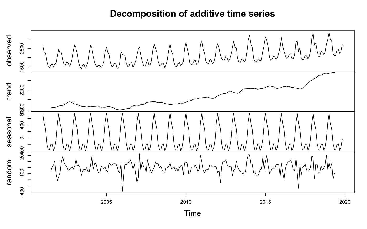
ts_seasonal(totalgasusagets,type="all")

Seasonal decomposition is another way to better understand pattens in the data. There are generally 3-4 components that can reconstitude the original series these are: Trend, Seasoan, Cycle and Irregular values. T/S/C/I.

These could be additive:

\[Y=T+S+C+I\]

or multiplicative:

\[Y=T*S*C*I\]

In most forecasting methods the variation in the series remain constant over time which is the case for additive series. However, sometimes the variation increase with time this where we need apply transformation to the data. Popular transformations are log or box-cox.

totalgasusagets_lambda=BoxCox.lambda(totalgasusagets)
df<-BoxCox(totalgasusagets,lambda = totalgasusagets_lambda)
ts_plot(df)

df<-decompose(totalgasusagets)
m<-plot(df)

m

## NULL

Auto Regressive Models

• Split data into training and testing
• train model using training
• Evaluate model statistics using both training and testing
• tune model if possible
• modify model paramters and choose a different model
• train and forecast using the full data set

Splitting

totalgasusagetspartition<-ts_split(totalgasusagets,sample.out = 12)
train<-totalgasusagetspartition$train
test<-totalgasusagetspartition$test

Forecasting

m<-auto.arima(train)

Forcast evaluation

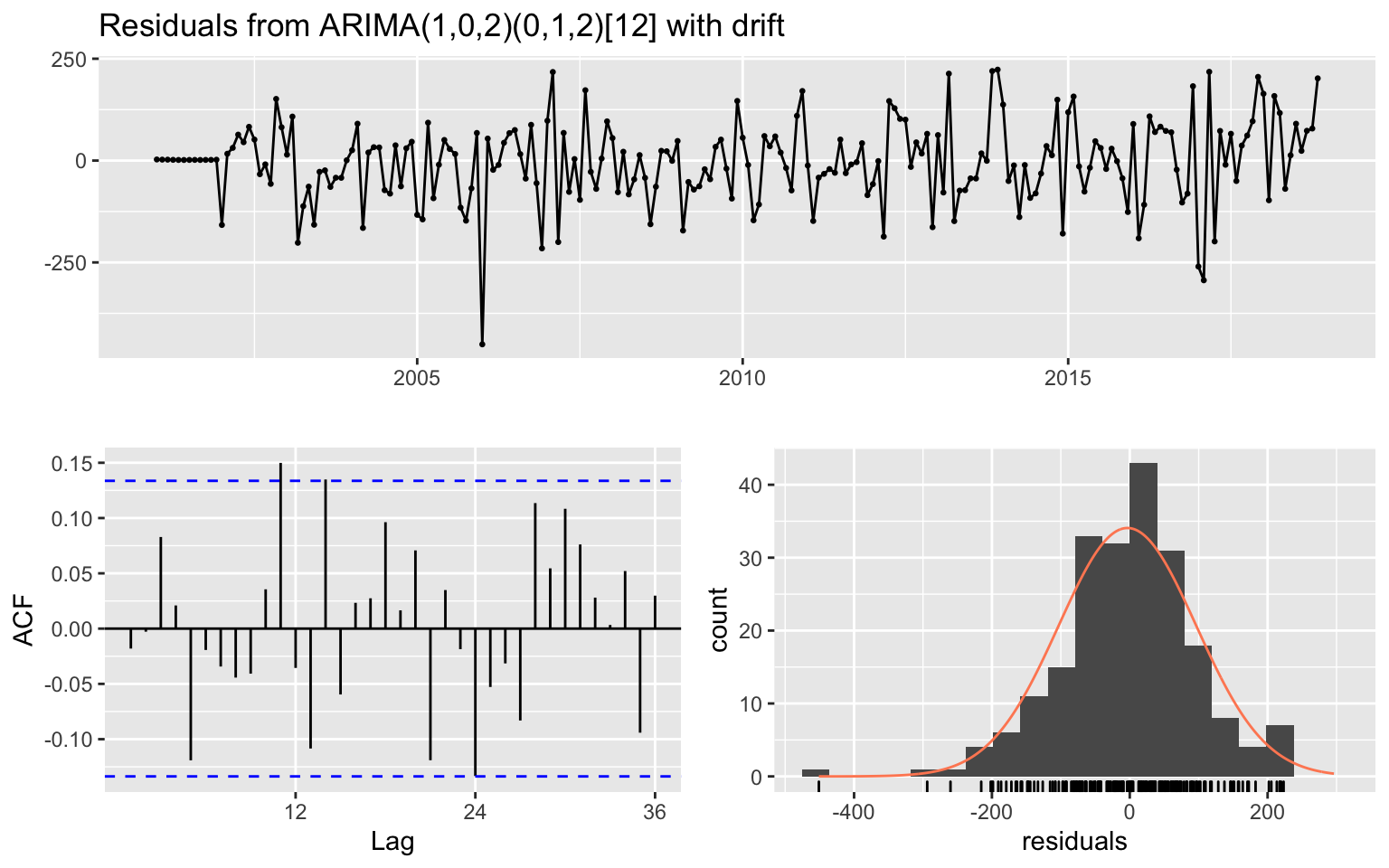
• Residual Analysis - Quality of the model + fitted values in the training partition
• Score forecast - How well model forecasts values

residual : \[e = Y_t- \bar{Y}_t\]

What we are looking for:

• Residuals are systematically higher/lower than zero
• Random spike - potential outliers
• Residual auto correlation - Seasonal pattern that is not captured by the model
• Residual distribution - need to be generally normal and spread shows the potential error in the model

checkresiduals(m)

## 
##  Ljung-Box test
## 
## data:  Residuals from ARIMA(1,0,2)(0,1,2)[12] with drift
## Q* = 31.369, df = 18, p-value = 0.02608
## 
## Model df: 6.   Total lags used: 24

Scoring the forecast:

• Mean Squared Error (MSE)
• Root mean squared error (RMSE)
• Mean absolute error (MAE)
• Mean absolute Percentage error (MAPE)

f<-forecast(m,h=12)

Accuracy is a relative metric what we are interested here is to understand if we get fairly consistent accuracy between training and test set. Overall 3% for MAPE is fairly good

accuracy(f,test)

##                     ME     RMSE      MAE        MPE     MAPE      MASE
## Training set -3.372419 99.68471 74.81482 -0.3675811 3.571766 0.6450949
## Test set      8.077045 95.58541 79.81804  0.2564342 3.187882 0.6882355
##                     ACF1 Theil's U
## Training set -0.01805577        NA
## Test set      0.18743721 0.2835977

Now putting it all together we can see actual vs. forecast and fitted data to do visual inspection of the results.

test_forecast(actual=totalgasusagets,forecast.obj = f,test = test)

Another way to assess the quality of the forecast to look at how much of variation in the forecast result can be explained by the model vs. mean of the data set.

meansvalue<-naive(train,n=12)
accuracy(meansvalue,test)

##                        ME     RMSE      MAE        MPE     MAPE     MASE
## Training set    0.1538551 287.4724 230.5047 -0.8777693 11.01401 1.987539
## Test set     -130.8745000 452.2096 421.3645 -7.9068138 17.09726 3.633239
##                   ACF1 Theil's U
## Training set 0.3689685        NA
## Test set     0.6614102  1.630007

Now finalize forecast

m_final<-auto.arima(totalgasusagets)
f_final<-forecast(m_final,h=12)

plot_forecast(f_final,
              title="US Natural Gas Consumption forecast",
              Xtitle = "Year",
              Ytitle = "BCF"
              
              )

We can use forecasting models to simulate values.

fc_sim<-forecast_sim(model=m_final,h=50,n=100)

Multiple forecasting models

We can also compare different forecasting methods

https://cran.r-project.org/web/packages/forecastHybrid/vignettes/forecast Hybrid.html

require(forecastHybrid)
hm1 <- hybridModel(y = totalgasusagets, models = "aefnstz", weights = "equal", errorMethod = "MASE")

accuracy(hm1,individual = T)

## $auto.arima
##                    ME     RMSE      MAE       MPE    MAPE      MASE
## Training set 10.41044 99.22508 74.44634 0.3593353 3.50313 0.6483263
##                     ACF1
## Training set -0.02563542
## 
## $ets
##                    ME     RMSE      MAE       MPE     MAPE      MASE
## Training set 4.385284 102.8923 78.79254 0.1557682 3.736481 0.6861757
##                   ACF1
## Training set 0.0479267
## 
## $thetam
##                    ME     RMSE      MAE       MPE     MAPE    MASE
## Training set 2.248873 386.8789 330.8795 -3.050205 15.82328 2.88151
##                   ACF1
## Training set 0.6911921
## 
## $nnetar
##                       ME     RMSE      MAE       MPE     MAPE      MASE
## Training set -0.07172379 126.2052 97.23931 -0.349635 4.617908 0.8468219
##                   ACF1
## Training set 0.2933973
## 
## $stlm
##                    ME     RMSE      MAE       MPE     MAPE      MASE
## Training set 6.757119 92.09597 68.74729 0.1714793 3.275024 0.5986953
##                    ACF1
## Training set 0.09310134
## 
## $tbats
##                   ME     RMSE      MAE       MPE     MAPE      MASE
## Training set 8.21607 100.8596 74.92726 0.1918939 3.564934 0.3236068
##                    ACF1
## Training set 0.07600191
## 
## $snaive
##                    ME     RMSE      MAE      MPE     MAPE MASE     ACF1
## Training set 39.89407 147.3022 114.8285 1.635774 5.385721    1 0.461255

Regression Forecasting

The final approach to forecasting is regression forecasting. The general formulation for regression (linear) looks like:

\[Y=B_0+B_1X_1+B_2X_2+B_3X_3...+B_nX_n+e\]

The most common estimation is OLS.

The assumptions in OLS

• the model coefficients follow a linear structure
• No prefect col-linearity - one variable can not be linear combination of others
• Independent variable should not have zero variance
• error term is a “normal distribution” with mu=0
• both independent and dependent variables draw from the population in a random sample

df<-decompose(totalgasusagets)

seasonal<-timetk::tk_tbl(df$seasonal,rename_index="date") %>% dplyr::rename(seasonal=value)
trend<-timetk::tk_tbl(df$trend,rename_index="date")%>% dplyr::rename(trend=value)
values<-timetk::tk_tbl(df$x,rename_index="date") %>% dplyr::rename(values=value)

all<-values %>% dplyr::left_join(seasonal,by="date") %>%
  dplyr::left_join(trend,by="date") %>% na.omit()

m<-lm(values~seasonal+trend,data=all[1:200,])
summary(m)

## 
## Call:
## lm(formula = values ~ seasonal + trend, data = all[1:200, ])
## 
## Residuals:
##     Min      1Q  Median      3Q     Max 
## -379.47  -53.53    3.79   57.64  235.58 
## 
## Coefficients:
##              Estimate Std. Error t value Pr(>|t|)    
## (Intercept) -23.67053   78.02601  -0.303    0.762    
## seasonal      0.99308    0.01753  56.647   <2e-16 ***
## trend         1.01127    0.03837  26.354   <2e-16 ***
## ---
## Signif. codes:  0 '***' 0.001 '**' 0.01 '*' 0.05 '.' 0.1 ' ' 1
## 
## Residual standard error: 93.38 on 197 degrees of freedom
## Multiple R-squared:  0.9528, Adjusted R-squared:  0.9524 
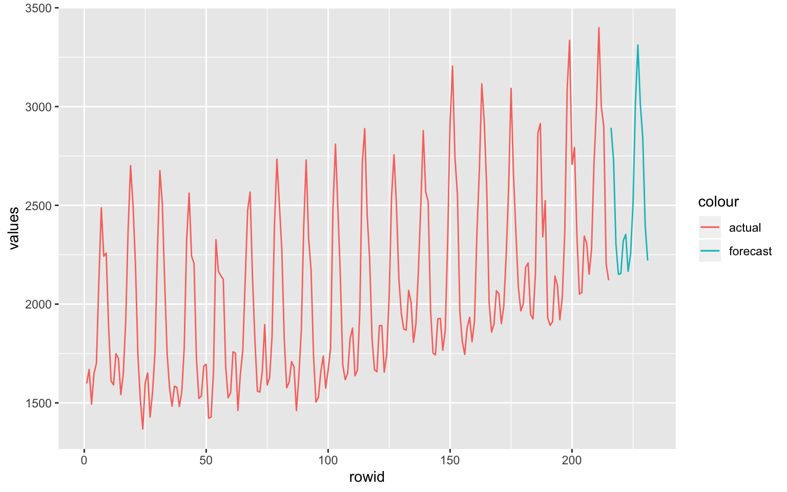
## F-statistic:  1991 on 2 and 197 DF,  p-value: < 2.2e-16

f<-forecast(m,newdata = all[200:215,],h = 20)
f

##    Point Forecast    Lo 80    Hi 80    Lo 95    Hi 95
##  1       2892.339 2769.900 3014.778 2704.558 3080.120
##  2       2731.155 2608.818 2853.492 2543.532 2918.779
##  3       2301.751 2179.280 2424.221 2113.923 2489.579
##  4       2150.776 2027.859 2273.694 1962.263 2339.290
##  5       2155.111 2032.079 2278.143 1966.421 2343.800
##  6       2321.283 2198.476 2444.090 2132.939 2509.627
##  7       2352.525 2229.587 2475.463 2163.980 2541.071
##  8       2165.841 2042.472 2289.210 1976.634 2355.048
##  9       2253.724 2130.508 2376.940 2064.752 2442.696
## 10       2505.457 2382.480 2628.435 2316.851 2694.063
## 11       3023.129 2899.692 3146.566 2833.818 3212.440
## 12       3311.735 3187.555 3435.916 3121.285 3502.186
## 13       3012.001 2888.475 3135.526 2822.554 3201.447
## 14       2840.290 2716.929 2963.652 2651.095 3029.485
## 15       2395.503 2272.120 2518.885 2206.276 2584.729
## 16       2220.805 2097.188 2344.422 2031.218 2410.392

nall<-data.frame(f) %>% dplyr::rename(values=`Point.Forecast`)
a<-all %>% dplyr::select(values) %>% bind_rows(nall) %>%
  dplyr::select(values) %>% tibble::rowid_to_column()

a %>% ggplot()+geom_line(aes(x=rowid,y=values,color="actual"),data=a[1:215,])+geom_line(aes(x=rowid,y=values,color="forecast"),data=a[216:231,])

While this method can seem counter intuitive and containing more steps but it provide a great deal of flexibility around independent variables. Forexample one can include additional regressors such as price in the model. Create sensitivity scenarios around some of the variables such as trend which will make the model good for both forecasting as well as explaining dynamics.

There is a new package by Rami Krispin forecastLM - some of the concepts are also convered in his book Hands-om Time-Series Analysis with R

There is a fantastic corresponding blogpost Introduction to the forecastLM package

References

[1] Github for the training sessions github

[2] Forecasting Principles and Practive - Rob J Hyndman and George Athanasopoulos

[3] [Hands-On Time Series Analysis with R: Perform time series analysis and forecasting using R by Rami Krispin] (https://www.amazon.ca/Hands-Time-Analysis-forecasting-visualization-ebook/dp/B07B41P2HZ)